§ 13. Basics of Monte Carlo¶
Monte Carlo Estimation¶
Definition 13.1 : Monte Carlo Estimation
Consider IID data \(X_{1}, \ldots, X_{N} \sim f\). Let \(\phi(X) \geq 0\) be some function. (The assumption \(\phi(X) \geq 0\) can be relaxed.) Consider the problem of estimating
One commonly uses
to estimate \(I\), which is called monte carlo estimation. After all, \(\mathbb{E}\left[\hat{I}_{N}\right]=I\) and \(\hat{I}_{N} \rightarrow I\) by the law of large numbers. (Convergence in probability by weak law of large numbers and almost sure convergence by strong law of large numbers.)
Concept 13.2 : Evidence of Convergence for Monte Carlo Estimation
We can quantify convergence with variance:
In other words
and
as \(N \rightarrow \infty\). So, \(\hat{I}_{N} \rightarrow I\) in \(L^2\) provided that \(\operatorname{Var}_{X \sim f}(\phi(X)) < \infty\).
Definition 13.3 : Empirical Risk Minimization (ERM)
In machine learning and statistics, we often wish to solve
where the objective function
Is the (true) risk. However, the evaluation of \(\mathbb{E}_{X \sim p_{X}}\) is impossible (if \(p_{X}\) is unknown) or intractable (if \(p_{X}\) is known but the expectation has no closed-form solution). Therefore, we define the proxy loss function
which we call the empirical risk, and solve
This is called empirical risk minimization (ERM). The idea is that
with high probability, so minimizing \(\mathcal{L}_{N}(\theta)\) should be similar to minimizing \(\mathcal{L}(\theta)\).
Concept 13.4 : Evidence of Convergence for Empirical Risk Minimization
Technical note) The law of large numbers tells us that
for any given \(\theta\), but we need
for all compact \(\Theta\) in order to conclude that the argmins of the two losses to be similar. These types of results are established by a uniform law of large numbers.
Importance Sampling¶
Definition 13.5 : Importance Sampling (IS)
Importance sampling (IS) is a technique for reducing the variance of a Monte Carlo estimator.
Key insight of important sampling:
(We do have to be mindful of division by 0.) Then
with \(X_{1}, \ldots, X_{N} \sim g\) is also an estimator of \(I\). Indeed, \(\mathbb{E}\left[\hat{I}_{N}\right]=I\) and \(\hat{I}_{N} \rightarrow I\). The weight \(\frac{f(x)}{g(x)}\) is called the likelihood ratio or the Radon-Nikodym derivative.
So we can use samples from \(g\) to compute expectation with respect to \(f\).
Consider the setup of estimating the probability
where \(X \sim \mathcal{N}(0,1)\). If we use the regular Monte Carlo estimator
where \(X_{i} \sim \mathcal{N}(0,1)\), if \(N\) is not sufficiently large, we can have \(\hat{I}_{N}=0\). Inaccurate estimate.
If we use the IS estimator
where \(Y_{i} \sim \mathcal{N}(3,1)\), having \(\hat{I}_{N}=0\) is much less likely. Estimate is much more accurate.
Concept 13.7 : Optimal Sampling Distribution
Benefit of IS quantified by with variance:
If \(\operatorname{Var}_{X \sim g}\left(\frac{\phi(X) f(X)}{g(X)}\right)<\operatorname{Var}_{X \sim f}(\phi(X))\), then IS provides variance reduction.
We call \(g\) the importance or sampling distribution. Choosing \(g\) poorly can increase the variance. What is the best choice of \(g\) ?
The sampling distribution
makes \(\operatorname{Var}_{X \sim g}\left(\frac{\phi(X) f(X)}{g(X)}\right)=\operatorname{Var}_{X \sim g}(I)=0\) and therefore is optimal. (\(I\) serves as the normalizing factor that ensures the density \(g\) integrates to 1.)
Problem: Since we do not know the normalizing factor \(I\), the answer we wish to estimate, sampling from \(g\) is usually difficult.
Concept 13.8 : Optimized / Trained Sampling Distribution
Instead, we consider the optimization problem
and compute a suboptimal, but good, sampling distribution within a class of sampling distributions \(\mathcal{G}\). (In ML, \(\mathcal{G}=\left\{g_{\theta} \mid \theta \in \Theta\right\}\) is parameterized by neural networks.)
Importantly, this optimization problem does not require knowledge of \(I\).
How do we compute stochastic gradients?
Log-Derivative Trick¶
Definition 13.9 : Log-Derivative Trick
Generally, consider the setup where we wish to solve
with SGD. (Previous situation (Concept 13.8) had \(\theta\)-dependence both on and inside the expectation. For now, let's simplify the problem so that \(\phi\) does not depend on \(\theta\).)
Incorrect gradient computation:
Correct gradient computation:
Therefore, \(\phi(X) \nabla_{\theta} \log \left(f_{\theta}(X)\right)\) with \(X \sim f_{\theta}\) is a stochastic gradient of the loss function. This technique is called the log-derivative trick, the likelihood ratio gradient\(^{\#}\), or REINFORCE\(^{\star}\).
Formula with the log-derivative \(\left(\nabla_{\theta} \log (\cdot)\right)\) is convenient when dealing with Gaussians, or more generally exponential families, since the densities are of the form
(\({}^{\#}\)P. W. Glynn, Likelihood ratio gradient estimation for stochastic systems, Communications of the ACM, 1990.
\({}^{\star}\)R. J. Williams, Simple statistical gradient-following algorithms for connectionist reinforcement learning. Machine Learning, 1992.)
Example 13.10 : Log-Derivative Trick Example
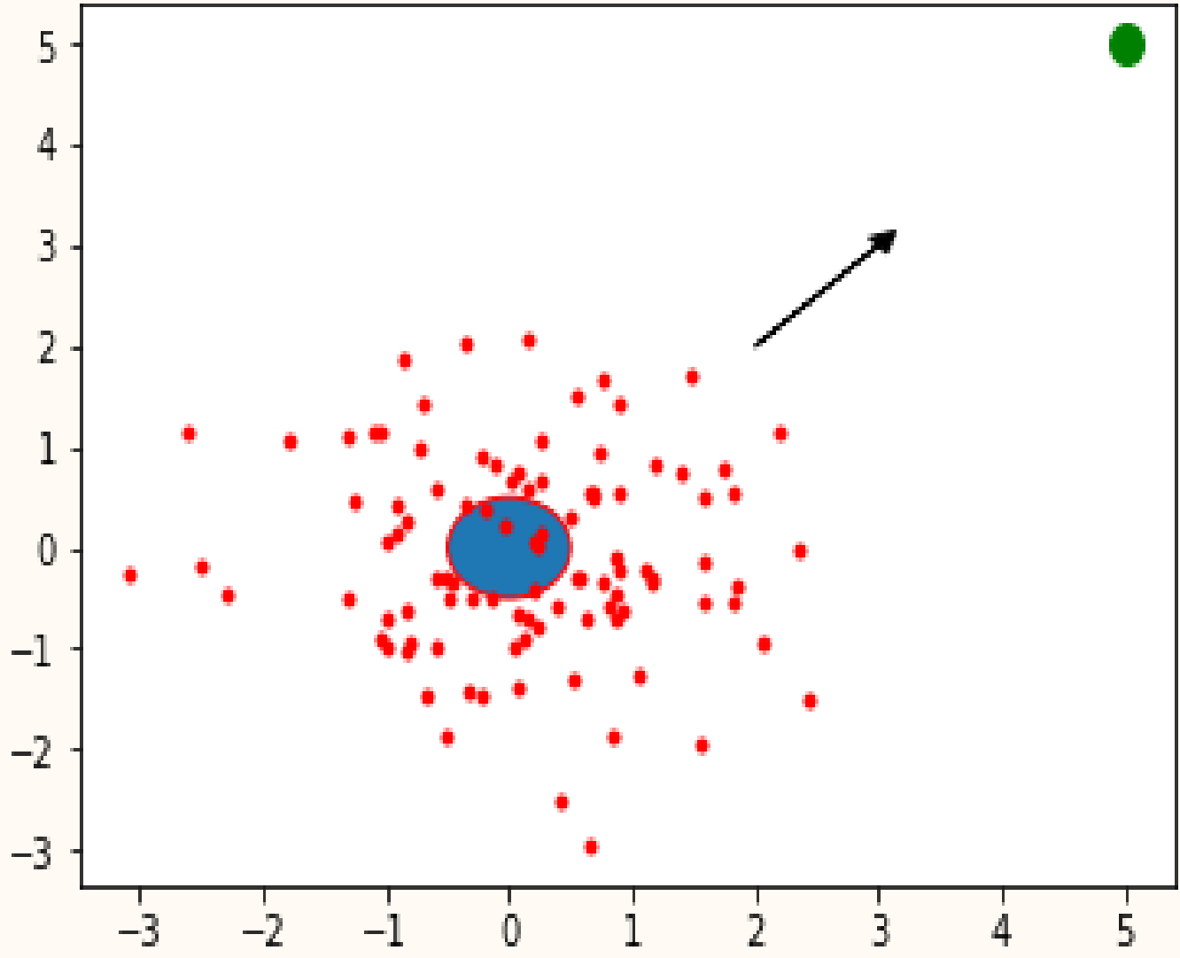
Learn \(\mu \in \mathbb{R}^{2}\) to minimize the objective below.
Then the loss function is
And, using \(X_{1}, \ldots, X_{B} \sim \mathcal{N}(\mu, I)\), we have stochastic gradients
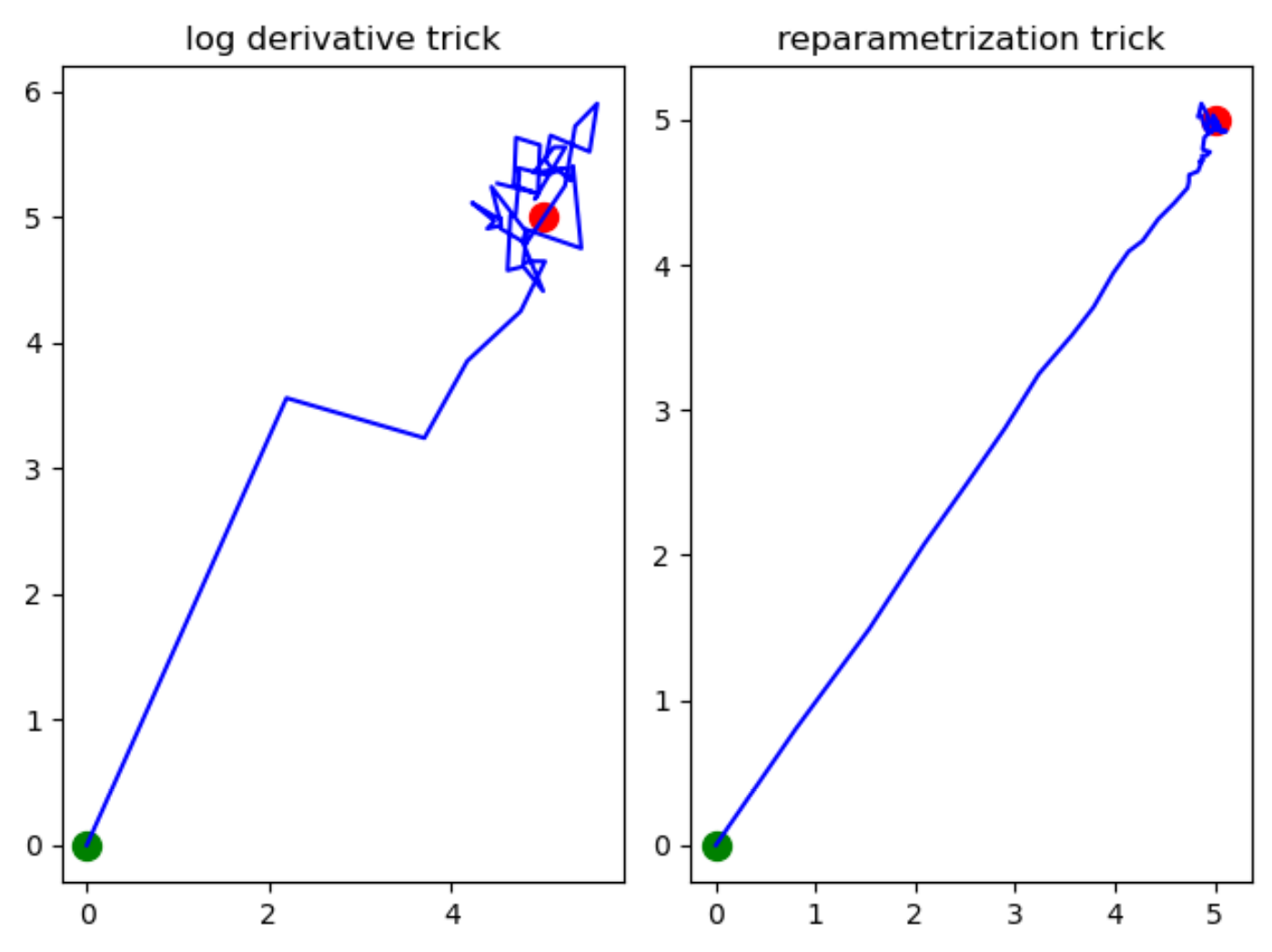
These stochastic gradients have large variance and thus SGD is slow.
Reparameterization Trick¶
Definition 13.11 : Reparameterization Trick
The reparameterization trick (RT) or the pathwise derivative (PD) relies on the key insight.
Gradient computation:
RT is less general than log-derivative trick, but it usually produces stochastic gradients with lower variance.
Example 13.12 : Reparameterization Trick Example
Consider the same example as before
Gradient computation:
These stochastic gradients have smaller variance and thus SGD is faster.
Example 13.13 : Log Derivative Trick vs Reparameterization Trick
The image below is the result of SGD with the computed gradients by Example 13.10 and Example 13.12.