§ 5. Convolutional Neural Networks¶

Convolutional Layers¶

Concept 5.1 : Pros and Cons of Fully Connected Layers

Advantages of fully connected layers:

Simple.
Very general, in theory. (Sufficiently large MLPs can learn any function, in theory.)

Disadvantage of fully connected layers:

Too many trainable parameters.
Does not encode shift equivariance/invariance and therefore has poor inductive bias. (More on this later.)

Concept 5.2 : Shift Equivarience/Invariance in Vision

Many tasks in vision are equivariant/invariant with respect shifts/translations.

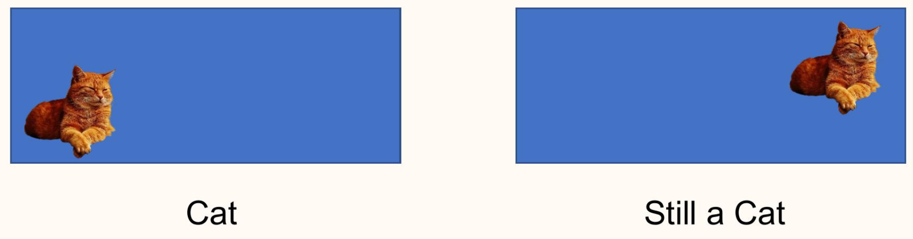
Roughly speaking, equivariance/invariance means shifting the object does not change the meaning (it only changes the position).

Logistic regression (with a single fully connected layer) does not encode shift invariance.

Since convolution is equivariant with respect to translations, constructing neural network layers with them is a natural choice.

Definition 5.3 : 2D Convolutional Layer

\(B\) : batch size
\(C_{\text{in}}\) : # of input channels
\(C_{\text{out}}\) : # of output channels
\(m, n\) : # of vertical and horizontal indices of input
\(f_1, f_2\) : # of vertical and horizontal indices of filter

Input tensor : \(X \in \mathbb{R}^{B \times C_{\text {in }} \times m \times n}\)
Output tensor : \(Y \in \mathbb{R}^{B \times C_{\text {out }} \times\left(m-f_{1}+1\right) \times\left(n-f_{2}+1\right)}\)
Filter : \(w \in \mathbb{R}^{C_{\text {out }} \times C_{\text {in }} \times f_{1} \times f_{2}}\)
Bias : \(b \in \mathbb{R}^{C_{\text{out}}}\)

For \(k = 1, \dots, B, \quad \ell = 1, \dots, C_{\text{out}}, \quad i = 1, \dots, m-f_1+1, \quad j = 1, \dots, n-f_2+1\):

\[ Y_{k, \ell, i, j}=\sum_{\gamma=1}^{c_{\text {in }}} \sum_{\alpha=1}^{f_{1}} \sum_{\beta=1}^{f_{2}} w_{\ell, \gamma, \alpha, \beta} X_{k, \gamma, i+\alpha-1, j+\beta-1}+b_{\ell} \]

Operation is independent across elements of the batch. The vertical and horizontal indices are referred to as spatial dimensions. If bias=False, then \(b=0\).

Convolve a filter with an image : slide the filter spatially over the image and compute dot products.

Take a \(C_{\text {in }} \times f_{1} \times f_{2}\) chunk of the image and take the inner product with \(w\) and add bias \(b\).

Example 5.4 : Example of 2D Convolutional Layer

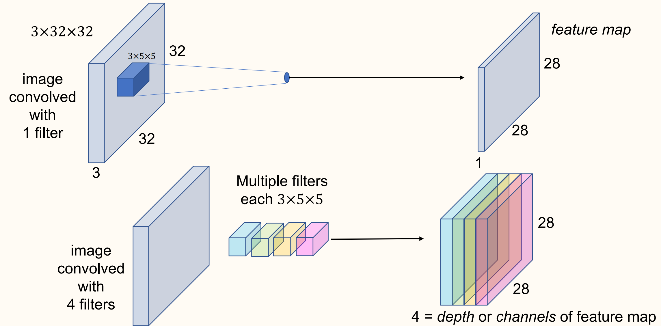
\(B = 1, C_{\text{in}} = 3, C_{\text{out}} = 4, m=n=32, f_1=f_2=5\)
Input tensor : \(X \in \mathbb{R}^{1 \times 3 \times 32 \times 32}\)
Output tensor : \(Y \in \mathbb{R}^{1 \times 4 \times 28 \times 28}\)
Filter : \(w \in \mathbb{R}^{4 \times 3 \times 5 \times 5}\)
Bias : \(b \in \mathbb{R}^{4}\)

Concept 5.5 : Zero Padding

Problem

Spatial dimension is reduced when passed through convolutional layers.

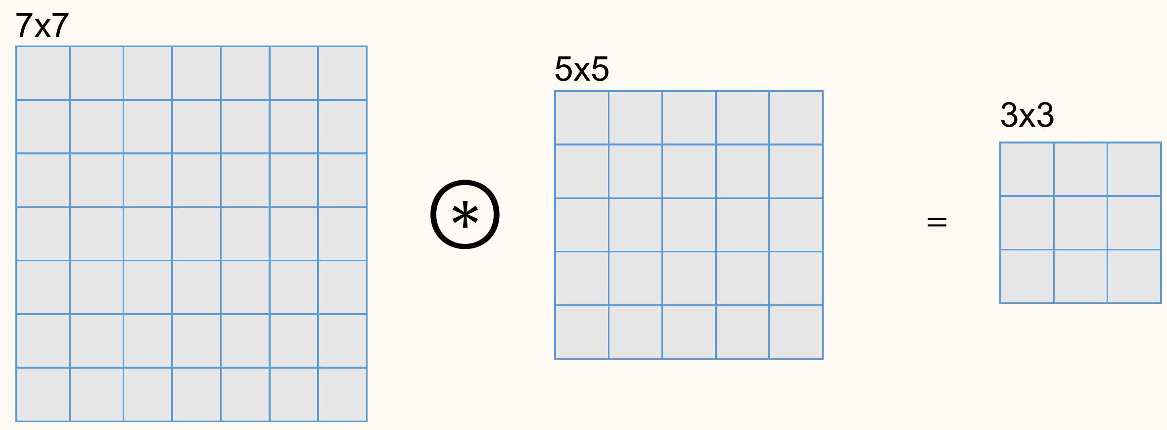
\((C \times 7 \times 7\) image\() \circledast(C \times 5 \times 5\) filter\()=(1 \times 3 \times 3\) feature map\()\). Spatial dimension 7 reduced to 3.

Solution

Zero padding on boundaries can preserve spatial dimension through convolutional layers.

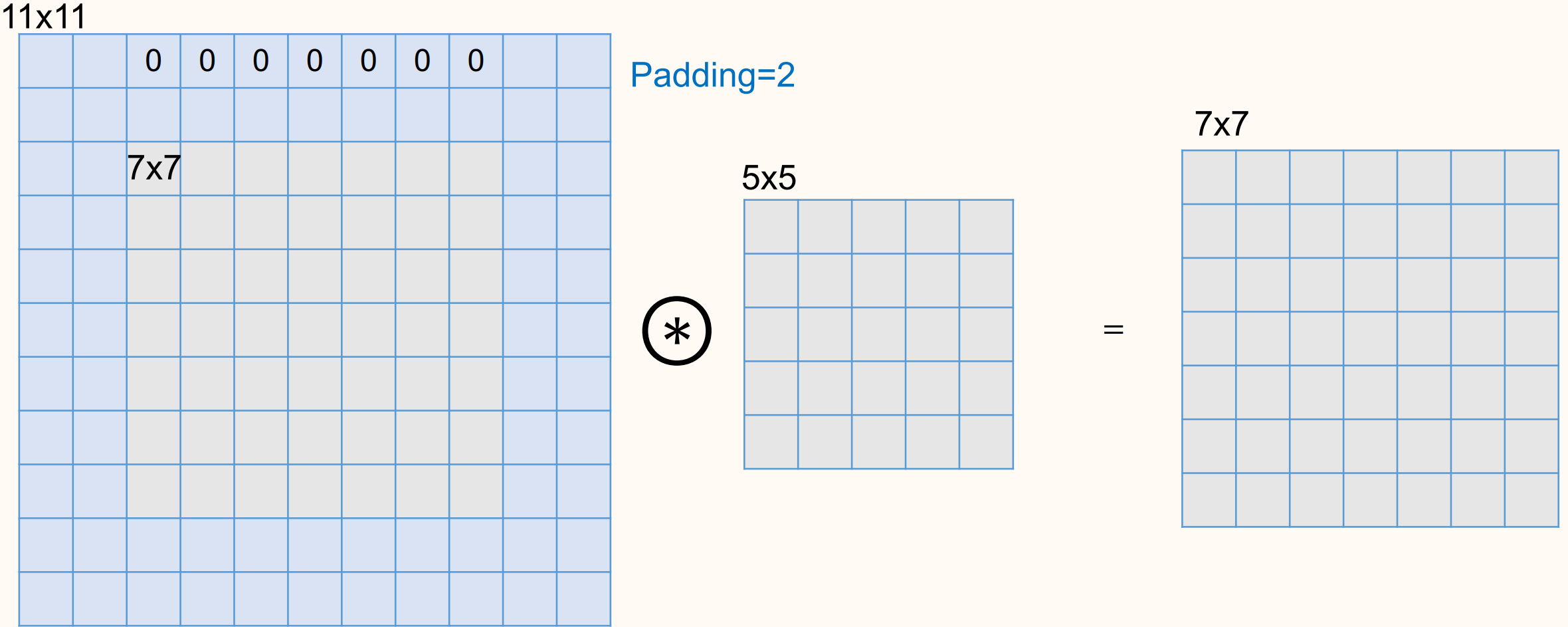
\((C \times 7 \times 7\) image with zero padding \(=2) \circledast(C \times 5 \times 5\) filter\()=(1 \times 7 \times 7\) feature map\()\). Spatial dimension is preserved.

Concept 5.6 : Stride

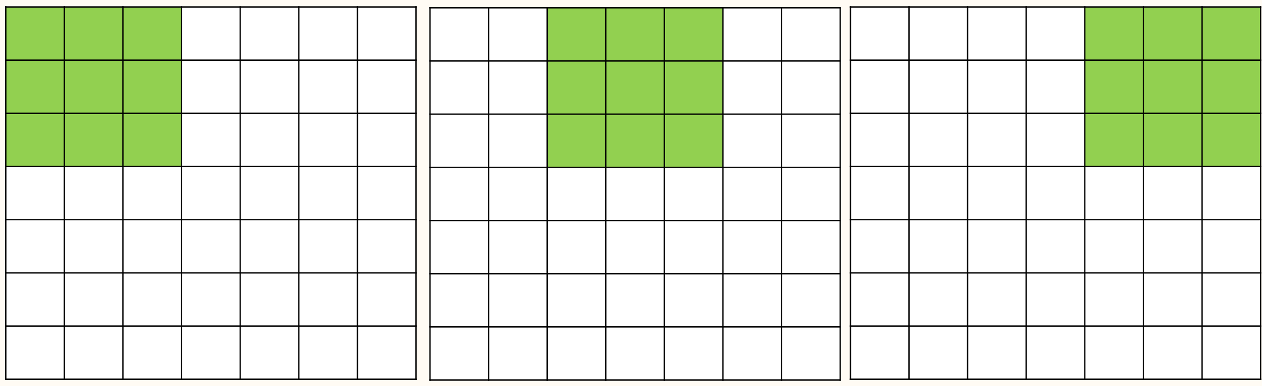
The horizontal/vertical distance of two adjacent inner product calculations with the filter when sliding it across the image is called stride. It is originally set to 1, but can be adjusted.

\((7 \times 7\) image\() \circledast(3 \times 3\) filter\()\) with stride \(1=(\)output \(5 \times 5)\)
\((7 \times 7\) image\() \circledast(3 \times 3\) filter\()\) with stride \(2=(\)output \(3 \times 3)\)
\((7 \times 7\) image with zero padding \(=1) \circledast(3 \times 3\) filter\()\) with stride \(3=(\)output \(3 \times 3)\)

Concept 5.7 : Convolution Summary

Input tensor : \(C_{\text {in}} \times W_{\text {in}} \times H_{\text {in}}\)
Convolution Layer parameters
- \(C_{\text {out}}\) filters, each of \(C_{\text {in}} \times F \times F\)
- Stride : \(S\)
- Padding : \(P\)
Output tensor : \(C_{\text {out}} \times W_{\text {out}} \times H_{\text {out}}\)

\[ \begin{aligned} & W_{\text{out}}=\left\lfloor\frac{W_{\text{in}}-F+2 P}{S}+1\right\rfloor \\ & H_{\text{out}}=\left\lfloor\frac{H_{\text{in}}-F+2 P}{S}+1\right\rfloor \end{aligned} \]

To avoid the complication of this floor operation, it is best to ensure the formula inside evaluates to an integer.
Number of trainable parameters : \(F^2 C_{\text{in}} C_{\text{out}}\) (filters) \(+ C_{\text{out}}\) (biases)

Concept 5.8 : Pooling

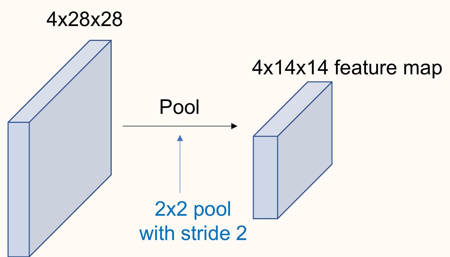
Pooling is primarily used to reduce spatial dimension. Similar to convolution. Pooling operates over each channel independently.

Concept 5.9 : Weight Sharing

In neural networks, weight sharing is a way to reduce the number of parameters by reusing the same parameter in multiple operations. Convolutional layers are the primary example.

\[ A_{w}=\left[\begin{array}{cccccccc} w_{1} & \cdots & w_{r} & 0 & \cdots & & & 0 \\ 0 & w_{1} & \cdots & w_{r} & 0 & \cdots & & 0 \\ 0 & 0 & w_{1} & \cdots & w_{r} & 0 & \cdots & 0 \\ \vdots & & & \ddots & & \ddots & & \vdots \\ 0 & & \cdots & 0 & w_{1} & \cdots & w_{r} & 0 \\ 0 & & \cdots & 0 & 0 & w_{1} & \cdots & w_{r} \end{array}\right] \]

If we consider convolution with filter \(w\) as a linear operator, the components of \(w\) appear may times in the matrix representation. This is because the same \(w\) is reused for every patch in the convolution. Weight sharing in convolution may now seem obvious, but it was a key contribution back when the LeNet architecture was presented.

Some models (not studied in this course) use weight sharing more explicitly in other ways.

Concept 5.10 : Geometric Deep Learning

More generally, given a group \(\mathcal{G}\) encoding a symmetry or invariance, one can define operations "equivariant" with respect \(\mathcal{G}\) and construct equivariant neural networks.

This is the subject of geometric deep learning, and its formulation utilizes graph theory and group theory.

Geometric deep learning is particularly useful for non-Euclidean data. Examples include as protein molecule data and social network service connections.