§ 19. Determinants of Order 2¶
Definition and Properties of Determinants of Order 2¶
Definition 19.1 : Determinant of a \(2 \times 2\) Matrix
If
is a \(2 \times 2\) matrix with entries from a field \(F\), then we define the determinant of \(A\), denoted \(\operatorname{det}(A)\) or \(|A|\), to be the scalar \(a d-b c\).
Theorem 19.2 : Linearity of determinant in each row
The function \(\operatorname{det}: \mathrm{M}_{2 \times 2}(F) \rightarrow F\) is a linear function of each row of a \(2 \times 2\) matrix when the other row is held fixed. That is, if \(u\), \(v\), and \(w\) are in \(F^{2}\) and \(k\) is a scalar, then
and
Proof
Let \(u=\left(a_{1}, a_{2}\right), v=\left(b_{1}, b_{2}\right)\), and \(w=\left(c_{1}, c_{2}\right)\) be in \(F^{2}\) and \(k\) be a scalar. Then
A similar calculation shows that
Theorem 19.3 : Invertibility and the determinant
Let \(A \in \mathrm{M}_{2 \times 2}(F)\). Then the determinant of \(A\) is nonzero if and only if \(A\) is invertible. Moreover, if \(A\) is invertible, then
Proof
If \(\operatorname{det}(A) \neq 0\), then we can define a matrix
A straightforward calculation shows that \(A M=M A=I\), and so \(A\) is invertible and \(M=A^{-1}\).
Conversely, suppose that \(A\) is invertible. Theorem 16.2 shows that the rank of
must be 2. Hence \(A_{11} \neq 0\) or \(A_{21} \neq 0\). If \(A_{11} \neq 0\), add \(-A_{21} / A_{11}\) times row 1 of \(A\) to row 2 to obtain the matrix
Because elementary row operations are rank-preserving by Corollary 16.5, it follows that
Therefore \(\operatorname{det}(A)=A_{11} A_{22}-A_{12} A_{21} \neq 0\). On the other hand, if \(A_{21} \neq 0\), we see that \(\operatorname{det}(A) \neq 0\) by adding \(-A_{11} / A_{21}\) times row 2 of \(A\) to row 1 and applying a similar argument. Thus, in either case, \(\operatorname{det}(A) \neq 0\).
Theorem 19.4 : Characterization of the \(2 \times 2\) determinant
Let \(\delta: \mathrm{M}_{2 \times 2}(F) \rightarrow F\) be a function with the following three properties.
- (a) \(\delta\) is a linear function of each row of the matrix when the other row is held fixed.
- (b) If the two rows of \(A \in \mathrm{M}_{2 \times 2}(F)\) are identical, then \(\delta(A)=0\).
- (c) If \(I\) is the \(2 \times 2\) identity matrix, then \(\delta(I)=1\).
Prove that \(\delta(A)=\operatorname{det}(A)\) for all \(A \in \mathrm{M}_{2 \times 2}(F)\).
Proof
Let
Write the first row as \(a(1,0)+b(0,1)\) and the second row as \(c(1,0)+d(0,1)\). Using (a) twice, \(\delta\) is linear in each row, so
By (b), the first and last terms are zero (the two rows are identical), so
By (c),
To compute \(\delta\!\left(\begin{array}{cc} 0 & 1 \\ 1 & 0 \end{array}\right)\), apply (b) to the matrix whose two rows are both \((1,1)\):
Using (a) to expand in the first row and then the second row gives
because the two remaining terms have identical rows and vanish by (b). Hence
so
Substituting back, we obtain
Theorem 19.2, Theorem 19.3, and Theorem 19.4 will be generalized to determinants of order \(n\) in section 22.
The Area of a Parallelogram¶
Definition 19.5 : Angle Between Two Vectors
By the angle between two vectors in \(\mathbb{R}^{2}\), we mean the angle with measure \(\theta(0 \leq \theta<\pi)\) that is formed by the vectors having the same magnitude and direction as the given vectors but emanating from the origin. (See Figure 19.1.)
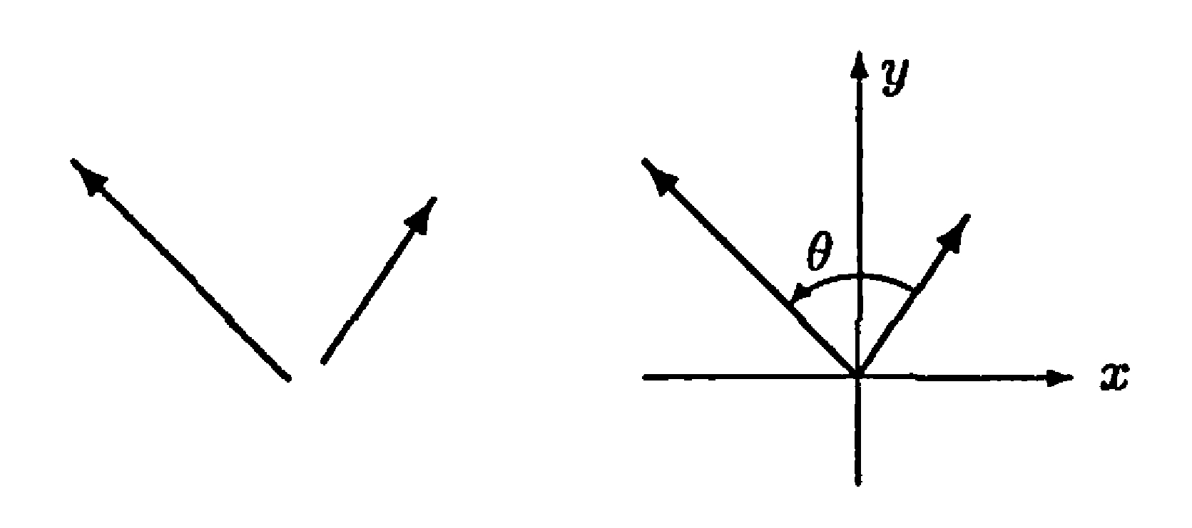
Figure 19.1: Angle between two vectors in \(\mathbb{R}^{2}\).
Definition 19.6 : Orientation of an Ordered Basis
If \(\beta=\{u, v\}\) is an ordered basis for \(\mathbb{R}^{2}\), we define the orientation of \(\beta\) to be the real number
(The denominator of this fraction is nonzero by Theorem 19.3.) Clearly
For convenience, we also define
if \(\{u, v\}\) is linearly dependent.
Definition 19.7 : Right-Handed and Left-Handed Coordinate Systems
Recall that a coordinate system \(\{u, v\}\) is called right-handed if \(u\) can be rotated in a counterclockwise direction through an angle \(\theta(0<\theta<\pi)\) to coincide with \(v\). Otherwise \(\{u, v\}\) is called a left-handed system.
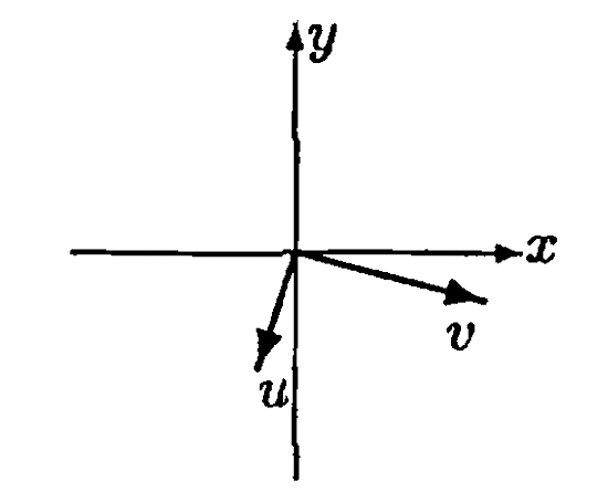
Figure 19.2: A right-handed coordinate system.
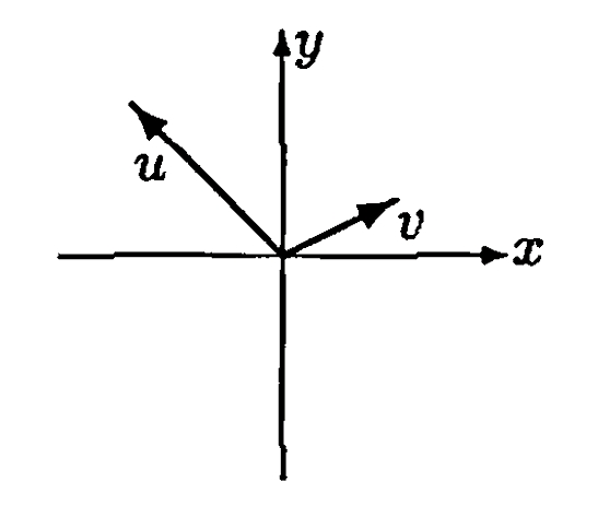
Figure 19.3: A left-handed coordinate system.
Theorem 19.8 : Orientation and right-handed coordinate systems
In general,
if and only if the ordered basis \(\{u, v\}\) forms a right-handed coordinate system.
Definition 19.9 : Parallelogram Determined by Two Vectors
Any ordered set \(\{u, v\}\) in \(\mathbb{R}^{2}\) determines a parallelogram in the following manner. Regarding \(u\) and \(v\) as arrows emanating from the origin of \(\mathbb{R}^{2}\), we call the parallelogram having \(u\) and \(v\) as adjacent sides the parallelogram determined by \(u\) and \(v\).
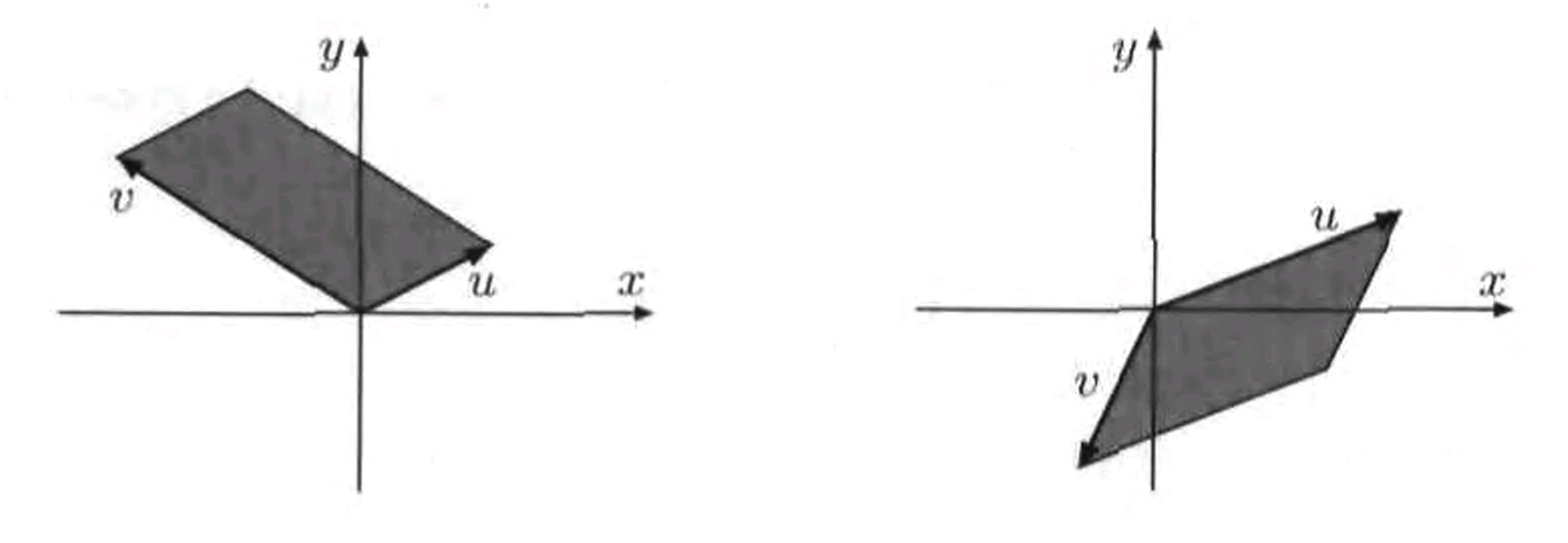
Figure 19.4.
Observe that if the set \(\{u, v\}\) is linearly dependent (i.e., if \(u\) and \(v\) are parallel), then the "parallelogram" determined by \(u\) and \(v\) is actually a line segment, which we consider to be a degenerate parallelogram having area zero.
We denote
the area of the parallelogram determined by \(u\) and \(v\).
Theorem 19.10 : Area of a parallelogram
from which it follows that
Proof
Our argument that
employs a technique that, although somewhat indirect, can be generalized to \(\mathbb{R}^{n}\). First, since
we may multiply both sides of the desired equation by
to obtain the equivalent form
We establish this equation by verifying that the three conditions of Theorem 19.4 are satisfied by the function
-
(a) We begin by showing that for any real number \(c\)
\[ \delta\binom{u}{c v}=c \cdot \delta\binom{u}{v} . \]Observe that this equation is valid if \(c=0\) because
\[ \delta\binom{u}{c v}=\mathrm{O}\binom{u}{0} \cdot \mathrm{~A}\binom{u}{0}=1 \cdot 0=0 \]So assume that \(c \neq 0\). Regarding \(c v\) as the base of the parallelogram determined by \(u\) and \(c v\), we see that
\[ \mathrm{A}\binom{u}{c v}=\text { base } \times \text { altitude }=|c|(\text { length of } v)(\text { altitude })=|c| \cdot \mathrm{A}\binom{u}{v} \]since the altitude \(h\) of the parallelogram determined by \(u\) and \(c v\) is the same as that in the parallelogram determined by \(u\) and \(v\). (see Figure 19.5)
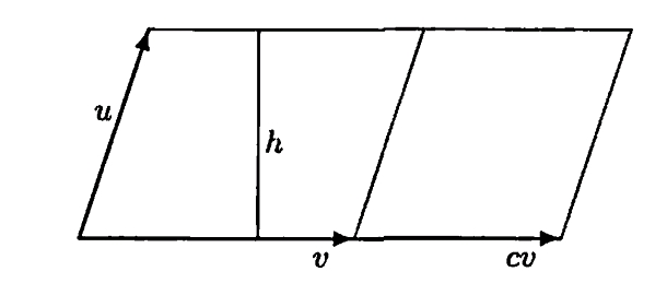
Figure 19.5.
Hence
\[ \begin{aligned} \delta\binom{u}{c v} & =\mathrm{O}\binom{u}{c v} \cdot \mathrm{~A}\binom{u}{c v}=\left[\frac{c}{|c|} \cdot \mathrm{O}\binom{u}{v}\right]\left[|c| \cdot \mathrm{A}\binom{u}{v}\right] \\ & =c \cdot \mathrm{O}\binom{u}{v} \cdot \mathrm{~A}\binom{u}{v}=c \cdot \delta\binom{u}{v} \end{aligned} \]A similar argument shows that
\[ \delta\binom{c u}{v}=c \cdot \delta\binom{u}{v} . \] -
(b) We next prove that
\[ \delta\binom{u}{a u+b w}=b \cdot \delta\binom{u}{w} \]for any \(u, w \in \mathbb{R}^{2}\) and any real numbers \(a\) and \(b\). Because the parallelograms determined by \(u\) and \(w\) and by \(u\) and \(u+w\) have a common base \(u\) and the same altitude (see Figure 19.6),
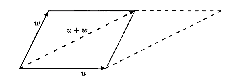
Figure 19.6.
it follows that
\[ \mathrm{A}\binom{u}{w}=\mathrm{A}\binom{u}{u+w} . \]If \(a=0\), then
\[ \delta\binom{u}{a u+b w}=\delta\binom{u}{b w}=b \cdot \delta\binom{u}{w} \]by the first paragraph of (a). Otherwise, if \(a \neq 0\), then
\[ \delta\binom{u}{a u+b w}=a \cdot \delta\binom{u}{u+\frac{b}{a} w}=a \cdot \delta\binom{u}{\frac{b}{a} w}=b \cdot \delta\binom{u}{w} . \]So the desired conclusion is obtained in either case. We are now able to show that
\[ \delta\binom{u}{v_{1}+v_{2}}=\delta\binom{u}{v_{1}}+\delta\binom{u}{v_{2}} \]for all \(u, v_{1}, v_{2} \in \mathbb{R}^{2}\). Since the result is immediate if \(u=0\), we assume that \(u \neq 0\). Choose any vector \(w \in \mathbb{R}^{2}\) such that \(\{u, w\}\) is linearly independent. Then for any vectors \(v_{1}, v_{2} \in \mathbb{R}^{2}\) there exist scalars \(a_{i}\) and \(b_{i}\) such that \(v_{i}=a_{i} u+b_{i} w(i=1,2)\). Thus
\[ \delta\binom{u}{v_{1}+v_{2}}=\delta\binom{u}{\left(a_{1}+a_{2}\right) u+\left(b_{1}+b_{2}\right) w}=\left(b_{1}+b_{2}\right) \delta\binom{u}{w} \]\[ =\delta\binom{u}{a_{1} u+b_{1} w}+\delta\binom{u}{a_{2} u+b_{2} w}=\delta\binom{u}{v_{1}}+\delta\binom{u}{v_{2}} . \]A similar argument shows that
\[ \delta\binom{u_{1}+u_{2}}{v}=\delta\binom{u_{1}}{v}+\delta\binom{u_{2}}{v} \]for all \(u_{1}, u_{2}, v \in \mathbb{R}^{2}\).
-
(c) Since
\[ \mathrm{A}\binom{u}{u}=0, \quad \text { it follows that } \quad \delta\binom{u}{u}=\mathrm{O}\binom{u}{u} \cdot \mathrm{~A}\binom{u}{u}=0 \]for any \(u \in \mathbb{R}^{2}\). Because the parallelogram determined by \(e_{1}\) and \(e_{2}\) is the unit square,
\[ \delta\binom{e_{1}}{e_{2}}=\mathrm{O}\binom{e_{1}}{e_{2}} \cdot \mathrm{~A}\binom{e_{1}}{e_{2}}=1 \cdot 1=1 \]
Therefore \(\delta\) satisfies the three conditions of Theorem 19.4, and hence \(\delta=\operatorname{det}\). So the area of the parallelogram determined by \(u\) and \(v\) equals
Example 19.11 : Area of a parallelogram
The area of the parallelogram determined by \(u=(-1,5)\) and \(v=(4,-2)\) is
Exercise¶
Exercise 19.10
The classical adjoint of a \(2 \times 2\) matrix \(A \in \mathrm{M}_{2 \times 2}(F)\) is the matrix
Prove that
- (a) \(C A=A C=[\operatorname{det}(A)] I\).
- (b) \(\operatorname{det}(C)=\operatorname{det}(A)\).
- (c) The classical adjoint of \(A^{t}\) is \(C^{t}\).
- (d) If \(A\) is invertible, then \(A^{-1}=[\operatorname{det}(A)]^{-1} C\).