§ 21. Properties of Determinants¶
Properties of Determinants¶
Theorem 21.1 : Determinants of elementary matrices
Because the determinant of the \(n \times n\) identity matrix is \(1\) (see Example 20.3), we can interpret Concept 20.12 as the following facts about the determinants of elementary matrices.
- (a) If \(E\) is an elementary matrix obtained by interchanging any two rows of \(I\), then \(\operatorname{det}(E)=-1\).
- (b) If \(E\) is an elementary matrix obtained by multiplying some row of \(I\) by the nonzero scalar \(k\), then \(\operatorname{det}(E)=k\).
- (c) If \(E\) is an elementary matrix obtained by adding a multiple of some row of \(I\) to another row, then \(\operatorname{det}(E)=1\).
Theorem 21.2 : Multiplicativity of the determinant
For any \(A, B \in \mathrm{M}_{n \times n}(F)\), \(\operatorname{det}(A B)=\operatorname{det}(A) \cdot \operatorname{det}(B)\).
Proof
We begin by establishing the result when \(A\) is an elementary matrix. If \(A\) is an elementary matrix obtained by interchanging two rows of \(I\), then \(\operatorname{det}(A)=-1\). But by Theorem 15.3, \(A B\) is a matrix obtained by interchanging two rows of \(B\). Hence by Theorem 20.12, \(\operatorname{det}(A B)=-\operatorname{det}(B)=\operatorname{det}(A) \cdot \operatorname{det}(B)\). Similarly, if \(A\) is an elementary matrix obtained by multiplying a row of \(I\) by a nonzero scalar \(k\), then \(\operatorname{det}(A)=k\), so \(\operatorname{det}(A B)=k \operatorname{det}(B)=\operatorname{det}(A) \cdot \operatorname{det}(B)\). Similarly, if \(A\) is an elementary matrix obtained by adding a multiple of one row of \(A\) to another row of \(A\), then \(\operatorname{det}(A)=1\), so \(\operatorname{det}(A B)=\operatorname{det}(B)=\operatorname{det}(A) \cdot \operatorname{det}(B)\).
If \(A\) is an \(n \times n\) matrix with rank less than \(n\), then \(\operatorname{det}(A)=0\) by Corollary 20.11 Since \(\operatorname{rank}(A B) \leq \operatorname{rank}(A)<n\) by Theorem 16.12, we have \(\operatorname{det}(A B)=0\). Thus \(\operatorname{det}(A B)=\operatorname{det}(A) \cdot \operatorname{det}(B)\) in this case.
On the other hand, if \(A\) has rank \(n\), then \(A\) is invertible and hence is the product of elementary matrices (Corollary 16.11), say, \(A=E_{m} \cdots E_{2} E_{1}\). The first paragraph of this proof shows that
Corollary 21.3 : Invertibility and the determinant
A matrix \(A \in \mathrm{M}_{n \times n}(F)\) is invertible if and only if \(\operatorname{det}(A) \neq 0\). Furthermore, if \(A\) is invertible, then \(\operatorname{det}\left(A^{-1}\right)=\frac{1}{\operatorname{det}(A)}\).
Proof
If \(A \in \mathrm{M}_{n \times n}(F)\) is not invertible, then the rank of \(A\) is less than \(n\). So \(\operatorname{det}(A)=0\) by Corollary 20.11. On the other hand, if \(A \in \mathrm{M}_{n \times n}(F)\) is invertible, then
by Theorem 21.2. Hence \(\operatorname{det}(A) \neq 0\) and \(\operatorname{det}\left(A^{-1}\right)=\frac{1}{\operatorname{det}(A)}\).
Theorem 21.4 : Determinant of a transpose
For any \(A \in \mathrm{M}_{n \times n}(F)\), \(\operatorname{det}\left(A^{t}\right)=\operatorname{det}(A)\).
Proof
If \(A\) is not invertible, then \(\operatorname{rank}(A)<n\). But \(\operatorname{rank}\left(A^{t}\right)=\operatorname{rank}(A)\) by Corollary 16.10, and so \(A^{t}\) is not invertible. Thus \(\operatorname{det}\left(A^{t}\right)=0=\operatorname{det}(A)\) in this case.
On the other hand, if \(A\) is invertible, then \(A\) is a product of elementary matrices, say \(A=E_{m} \cdots E_{2} E_{1}\). Since \(\operatorname{det}\left(E_{i}\right)=\operatorname{det}\left(E_{i}^{t}\right)\) for every \(i\) by Exercise 20.29, by Theorem 21.2 we have
Thus, in either case, \(\operatorname{det}\left(A^{t}\right)=\operatorname{det}(A)\).
Among the many consequences of Theorem 21.4 are that determinants can be evaluated by cofactor expansion along a column, and that elementary column operations can be used as well as elementary row operations in evaluating a determinant. (The effect on the determinant of performing an elementary column operation is the same as the effect of performing the corresponding elementary row operation.)
Cramer's Rule¶
Theorem 21.5 : Cramer's rule
Let \(A x=b\) be the matrix form of a system of \(n\) linear equations in \(n\) unknowns, where \(x=\left(x_{1}, x_{2}, \ldots, x_{n}\right)^{t}\). If \(\operatorname{det}(A) \neq 0\), then this system has a unique solution, and for each \(k\) (\(k=1,2, \ldots, n\)),
where \(M_{k}\) is the \(n \times n\) matrix obtained from \(A\) by replacing column \(k\) of \(A\) by \(b\).
Proof
If \(\operatorname{det}(A) \neq 0\), then the system \(A x=b\) has a unique solution by Corollary 21.3 and Theorem 17.6. For each integer \(k\) (\(1 \leq k \leq n\)), let \(a_{k}\) denote the \(k\)th column of \(A\) and \(X_{k}\) denote the matrix obtained from the \(n \times n\) identity matrix by replacing column \(k\) by \(x\). Then by Theorem 2.13 (p. 90), \(A X_{k}\) is the \(n \times n\) matrix whose \(i\)th column is
Thus \(A X_{k}=M_{k}\). Evaluating \(X_{k}\) by cofactor expansion along row \(k\) produces
Hence by Theorem 21.2,
Therefore
Example 21.6 : Solving a system by Cramer's rule
We illustrate Theorem 21.5 by using Cramer's rule to solve the following system of linear equations:
The matrix form of this system of linear equations is \(A x=b\), where
Because \(\operatorname{det}(A)=6 \neq 0\), Cramer's rule applies. Using the notation of Theorem 21.5, we have
and
Thus the unique solution to the given system of linear equations is
In applications involving systems of linear equations, we sometimes need to know that there is a solution in which the unknowns are integers. In this situation, Cramer's rule can be useful because it implies that a system of linear equations with integral coefficients has an integral solution if the determinant of its coefficient matrix is \(\pm 1\). On the other hand, Cramer's rule is not useful for computation because it requires evaluating \(n+1\) determinants of \(n \times n\) matrices to solve a system of \(n\) linear equations in \(n\) unknowns. Thus Cramer's rule is primarily of theoretical and aesthetic interest, rather than of computational value.
Geometric Interpretation of the Determinant¶
Definition 21.7 : Geometric Interpretation of the Determinant
As in Section 19, it is possible to interpret the determinant of a matrix \(A \in \mathrm{M}_{n \times n}(R)\) geometrically. If the rows of \(A\) are \(a_{1}, a_{2}, \ldots, a_{n}\), respectively, then \(|\operatorname{det}(A)|\) is the \(n\)-dimensional volume (the generalization of area in \(\mathbb{R}^{2}\) and volume in \(\mathbb{R}^{3}\)) of the parallelepiped having the vectors \(a_{1}, a_{2}, \ldots, a_{n}\) as adjacent sides.
Example 21.8 : Volume of a parallelepiped
The volume of the parallelepiped having the vectors \(a_{1}=(1,-2,1)\), \(a_{2}=(1,0,-1)\), and \(a_{3}=(1,1,1)\) as adjacent sides is
Note that the object in question is a rectangular parallelepiped (see Figure 21.1) with sides of lengths \(\sqrt{6}\), \(\sqrt{2}\), and \(\sqrt{3}\). Hence by the familiar formula for volume, its volume should be \(\sqrt{6} \cdot \sqrt{2} \cdot \sqrt{3}=6\), as the determinant calculation shows.
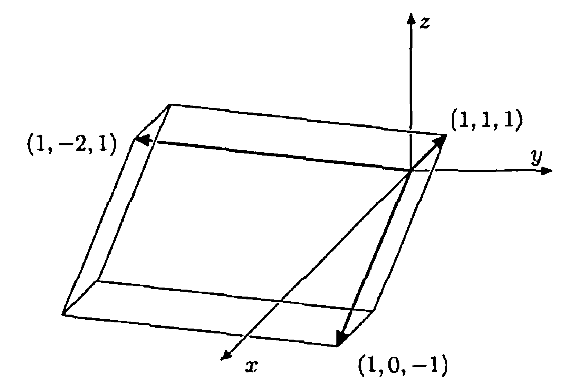
Figure 21.1.
Definition 21.9 : Right-Handed Coordinate Systems
If \(\gamma\) is any ordered basis for \(\mathbb{R}^{n}\) and \(\beta\) is the standard ordered basis for \(\mathbb{R}^{n}\), then \(\gamma\) induces a right-handed coordinate system if and only if \(\operatorname{det}(Q)>0\), where \(Q\) is the change of coordinate matrix changing \(\gamma\)-coordinates into \(\beta\)-coordinates.
Definition 21.10 : Orientation of Coordinate Systems
More generally, if \(\beta\) and \(\gamma\) are two ordered bases for \(\mathbb{R}^{n}\), then the coordinate systems induced by \(\beta\) and \(\gamma\) have the same orientation (either both are right-handed or both are left-handed) if and only if \(\operatorname{det}(Q)>0\), where \(Q\) is the change of coordinate matrix changing \(\gamma\)-coordinates into \(\beta\)-coordinates.
Example 21.11 : Orientation examples in \(\mathbb{R}^{3}\)
Thus, for instance,
induces a left-handed coordinate system in \(\mathbb{R}^{3}\) because
whereas
induces a right-handed coordinate system in \(\mathbb{R}^{3}\) because
Exercise¶
Exercise 21.10
A matrix \(M \in \mathrm{M}_{n \times n}(C)\) is called nilpotent if, for some positive integer \(k\), \(M^{k}=O\), where \(O\) is the \(n \times n\) zero matrix. Prove that if \(M\) is nilpotent, then \(\operatorname{det}(M)=0\).
Exercise 21.11
A matrix \(M \in \mathrm{M}_{n \times n}(C)\) is called skew-symmetric if \(M^{t}=-M\). Prove that if \(M\) is skew-symmetric and \(n\) is odd, then \(M\) is not invertible. What happens if \(n\) is even?
Exercise 21.12
A matrix \(Q \in \mathrm{M}_{n \times n}(R)\) is called orthogonal if \(Q Q^{t}=I\). Prove that if \(Q\) is orthogonal, then \(\operatorname{det}(Q)= \pm 1\).
Exercise 21.13
For \(M \in \mathrm{M}_{n \times n}(C)\), let \(\overline{M}\) be the matrix such that \((\overline{M})_{i j}=\overline{M_{i j}}\) for all \(i, j\), where \(\overline{M_{i j}}\) is the complex conjugate of \(M_{i j}\).
- (a) Prove that \(\operatorname{det}(\overline{M})=\overline{\operatorname{det}(M)}\).
- (b) A matrix \(Q \in \mathrm{M}_{n \times n}(C)\) is called unitary if \(Q Q^{*}=I\), where \(Q^{*}=\overline{Q^{t}}\). Prove that if \(Q\) is a unitary matrix, then \(|\operatorname{det}(Q)|=1\).
Exercise 21.15
Prove that if \(A, B \in \mathrm{M}_{n \times n}(F)\) are similar, then \(\operatorname{det}(A)=\operatorname{det}(B)\).
Exercise 21.17
Let \(A, B \in \mathrm{M}_{n \times n}(F)\) be such that \(A B=-B A\). Prove that if \(n\) is odd and \(F\) is not a field of characteristic two, then \(A\) or \(B\) is not invertible.
Exercise 21.20
Suppose that \(M \in \mathrm{M}_{n \times n}(F)\) can be written in the form
where \(A\) is a square matrix. Prove that \(\operatorname{det}(M)=\operatorname{det}(A)\).
Exercise 21.21
Prove that if \(M \in \mathrm{M}_{n \times n}(F)\) can be written in the form
where \(A\) and \(C\) are square matrices, then \(\operatorname{det}(M)=\operatorname{det}(A) \cdot \operatorname{det}(C)\).
Exercise 21.22
Let \(T: \mathrm{P}_{n}(F) \rightarrow F^{n+1}\) be the linear transformation defined in Exercise 22 of Section 2.4 by \(\mathrm{T}(f)=\left(f\left(c_{0}\right), f\left(c_{1}\right), \ldots, f\left(c_{n}\right)\right)\), where \(c_{0}, c_{1}, \ldots, c_{n}\) are distinct scalars in an infinite field \(F\). Let \(\beta\) be the standard ordered basis for \(\mathrm{P}_{n}(F)\). Let \(\gamma\) be the standard ordered basis for \(F^{n+1}\).
-
(a) Show that \(M=[T]_{\beta}^{\gamma}\) has the form
\[ \left(\begin{array}{ccccc} 1 & c_{0} & c_{0}^{2} & \cdots & c_{0}^{n} \\ 1 & c_{1} & c_{1}^{2} & \cdots & c_{1}^{n} \\ \vdots & \vdots & \vdots & & \vdots \\ 1 & c_{n} & c_{n}^{2} & \cdots & c_{n}^{n} \end{array}\right) . \]A matrix with this form is called a Vandermonde matrix.
-
(b) Use Exercise 22 of Section 2.4 to prove that \(\operatorname{det}(M) \neq 0\).
-
(c) Prove that
\[ \operatorname{det}(M)=\prod_{0 \leq i<j \leq n}\left(c_{j}-c_{i}\right) \]the product of all terms of the form \(c_{j}-c_{i}\) for \(0 \leq i<j \leq n\).
Exercise 21.23
Let \(A \in \mathrm{M}_{n \times n}(F)\) be nonzero. For any \(m\) (\(1 \leq m \leq n\)), an \(m \times m\) submatrix is obtained by deleting any \(n-m\) rows and any \(n-m\) columns of \(A\).
- (a) Let \(k\) (\(1 \leq k \leq n\)) denote the largest integer such that some \(k \times k\) submatrix has a nonzero determinant. Prove that \(\operatorname{rank}(A)=k\).
- (b) Conversely, suppose that \(\operatorname{rank}(A)=k\). Prove that there exists a \(k \times k\) submatrix with a nonzero determinant.
Exercise 21.24
Let \(A \in \mathrm{M}_{n \times n}(F)\) have the form
Compute \(\operatorname{det}(A+t I)\), where \(I\) is the \(n \times n\) identity matrix.
Exercise 21.25
Let \(c_{j k}\) denote the cofactor of the row \(j\), column \(k\) entry of the matrix \(A \in \mathrm{M}_{n \times n}(F)\).
- (a) Prove that if \(B\) is the matrix obtained from \(A\) by replacing column \(k\) by \(e_{j}\), then \(\operatorname{det}(B)=c_{j k}\).
-
(b) Show that for \(1 \leq j \leq n\), we have
\[ A\left(\begin{array}{c} c_{j 1} \\ c_{j 2} \\ \vdots \\ c_{j n} \end{array}\right)=\operatorname{det}(A) \cdot e_{j} \]Hint: Apply Cramer's rule to \(A x=e_{j}\).
-
(c) Deduce that if \(C\) is the \(n \times n\) matrix such that \(C_{i j}=c_{j i}\), then \(A C=[\operatorname{det}(A)] I\).
- (d) Show that if \(\operatorname{det}(A) \neq 0\), then \(A^{-1}=[\operatorname{det}(A)]^{-1} C\).
Definition 21.12 : Classical Adjoint of a Matrix
The classical adjoint of a square matrix \(A\) is the transpose of the matrix whose \(i j\)-entry is the \(i j\)-cofactor of \(A\).
Exercise 21.27
Let \(C\) be the classical adjoint of \(A \in \mathrm{M}_{n \times n}(F)\). Prove the following statements.
- (a) \(\operatorname{det}(C)=[\operatorname{det}(A)]^{n-1}\).
- (b) \(C^{t}\) is the classical adjoint of \(A^{t}\).
- (c) If \(A\) is an invertible upper triangular matrix, then \(C\) and \(A^{-1}\) are both upper triangular matrices.
Exercise 21.28
Let \(y_{1}, y_{2}, \ldots, y_{n}\) be linearly independent functions in \(\mathrm{C}^{\infty}\). For each \(y \in \mathrm{C}^{\infty}\), define \(\mathrm{T}(y) \in \mathrm{C}^{\infty}\) by
The preceding determinant is called the Wronskian of \(y, y_{1}, \ldots, y_{n}\).
- (a) Prove that \(\mathrm{T}: \mathrm{C}^{\infty} \rightarrow \mathrm{C}^{\infty}\) is a linear transformation.
- (b) Prove that \(N(T)\) contains \(\operatorname{span}\left(\left\{y_{1}, y_{2}, \ldots, y_{n}\right\}\right)\).